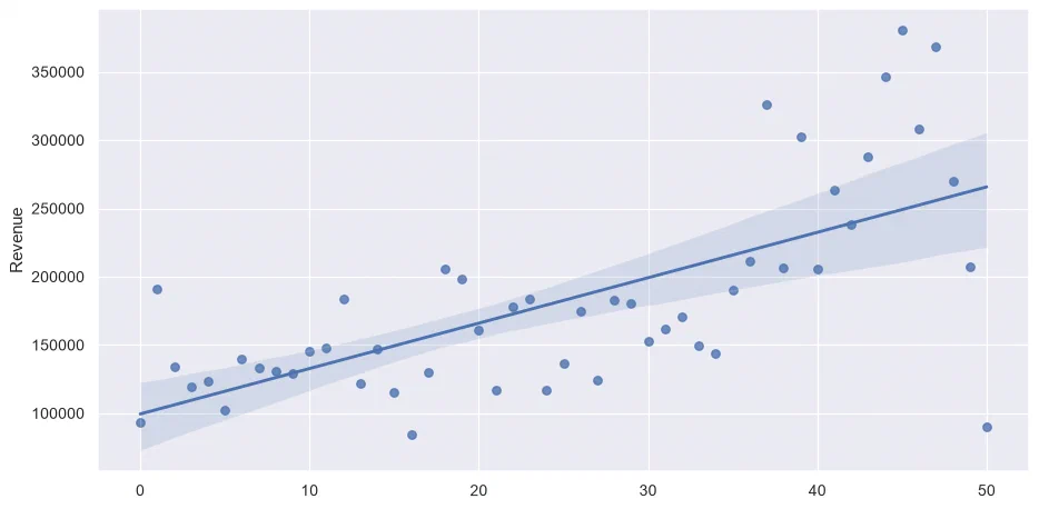
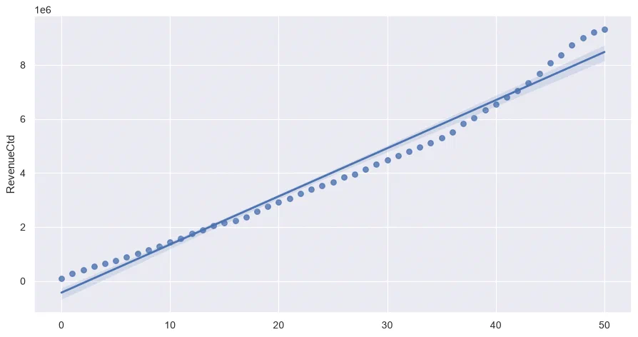
The dataset is Online Retail, from the UCI Machine Learning Repository: all the orders of a UK-based online shop selling gifts, mostly to wholesalers, from December 2010 to December 2011. One row is one product in one invoice, with its quantity, unit price, customer and country. Invoice numbers starting with a C are cancellations, with negative quantities.
It works well for teaching: real data, with its flaws (missing customers, returns, a few odd prices), about a business that everyone understands, and big enough (half a million rows) that a spreadsheet would struggle.
The course ended with a lifetime value model on the same data, which has its own post.
### Import standard librariesimportpandasaspdimportmatplotlib.pyplotaspltimportseabornassns### Setupsns.set(rc={'figure.figsize':(12,6)})
### Read source filedf=pd.read_excel("Online Retail.xlsx")### Change column typesdf['InvoiceDate']=pd.to_datetime(df['InvoiceDate'])df['Quantity']=df['Quantity'].astype('int')df['UnitPrice']=df['UnitPrice'].astype('float')df['CustomerID']=df['CustomerID'].astype('str')### Filter on 1 year of datadf=df.loc[lambdax:x['InvoiceDate']<'2011-12-01']
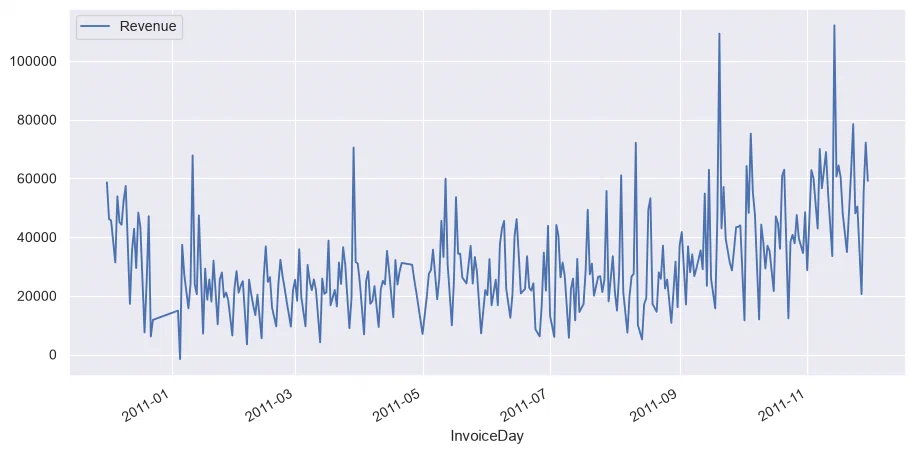
### First try to group by datedf_date=df.groupby('InvoiceDay').sum(numeric_only=True)df_date.head()
InvoiceDay
Quantity
UnitPrice
Week
WeekDay
Revenue
2010-12-01
26814
12904.25
149184
6216
58635.56
2010-12-02
21023
6815.68
101232
6327
46207.28
2010-12-03
14830
11114.09
105696
8808
45620.46
2010-12-05
16395
7893.17
130800
16350
31383.95
2010-12-06
21419
17678.78
190022
0
53860.18
### Let's try again with more appropriate aggregatesdf_date=(df.groupby('InvoiceDay').agg({'InvoiceNo':'nunique','CustomerID':'nunique','Quantity':'sum','Revenue':'sum'}).reset_index())df_date.head()
InvoiceDay
InvoiceNo
CustomerID
Quantity
Revenue
0
2010-12-01
143
98
26814
58635.56
1
2010-12-02
167
117
21023
46207.28
2
2010-12-03
108
55
14830
45620.46
3
2010-12-05
95
76
16395
31383.95
4
2010-12-06
133
90
21419
53860.18
### ✅ 4.1. Add back the UnitPricedf_date['UnitPrice']=df_date['Revenue']/df_date['Quantity']df_date.head()
InvoiceDay
InvoiceNo
CustomerID
Quantity
Revenue
UnitPrice
0
2010-12-01
143
98
26814
58635.56
2.19
1
2010-12-02
167
117
21023
46207.28
2.20
2
2010-12-03
108
55
14830
45620.46
3.08
3
2010-12-05
95
76
16395
31383.95
1.91
4
2010-12-06
133
90
21419
53860.18
2.51
### ✅ 4.2. Starting with `df`, get the revenue per countrydf.groupby('Country').agg({'Revenue':'sum'})
### ✅ 5.4. Group data by week in a dataframe named `df_week`### Don't forget to recompute the UnitPricedf_week=(df.groupby('Week').agg({'InvoiceNo':'nunique','CustomerID':'nunique','Quantity':'sum','Revenue':'sum'}).reset_index())df_week['UnitPrice']=df_week['Revenue']/df_week['Quantity']df_week.head()
Week
InvoiceNo
CustomerID
Quantity
Revenue
UnitPrice
0
1
320
236
73491
93720.93
1.28
1
2
343
235
85626
190994.96
2.23
2
3
297
214
67969
133782.91
1.97
3
4
431
274
69312
119136.81
1.72
4
5
384
270
67613
123642.18
1.83
### ✅ 5.5. What is the average revenue by week ?df_week['Revenue'].mean()
182629.01811764707
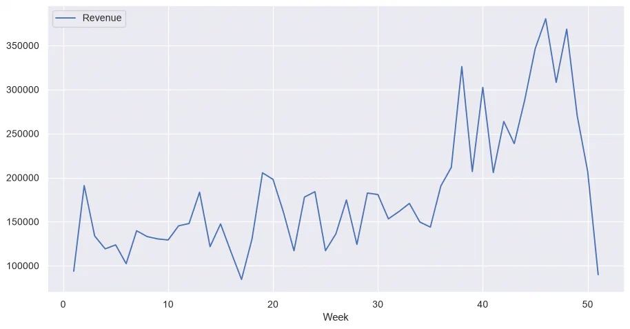
### ✅ 5.6. Plot the weekly Revenue evolutiondf_week.plot.line(x='Week',y='Revenue')
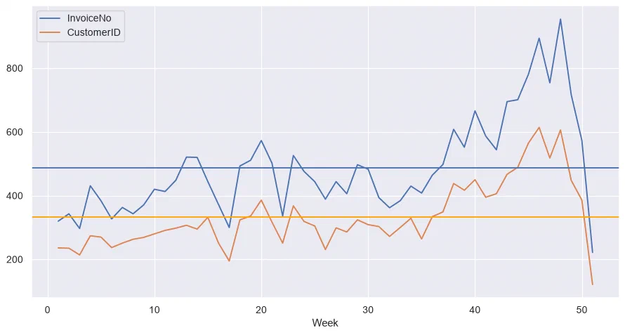
### ✅ 5.7. Now plot the weekly number of orders, along with the number of customers### and the average for each metric### Hint: use `ax.axhline()`fig,ax=plt.subplots()df_week.plot.line(x='Week',y='InvoiceNo',ax=ax)df_week.plot.line(x='Week',y='CustomerID',ax=ax)ax.axhline(df_week['InvoiceNo'].mean())ax.axhline(df_week['CustomerID'].mean(),color='orange')
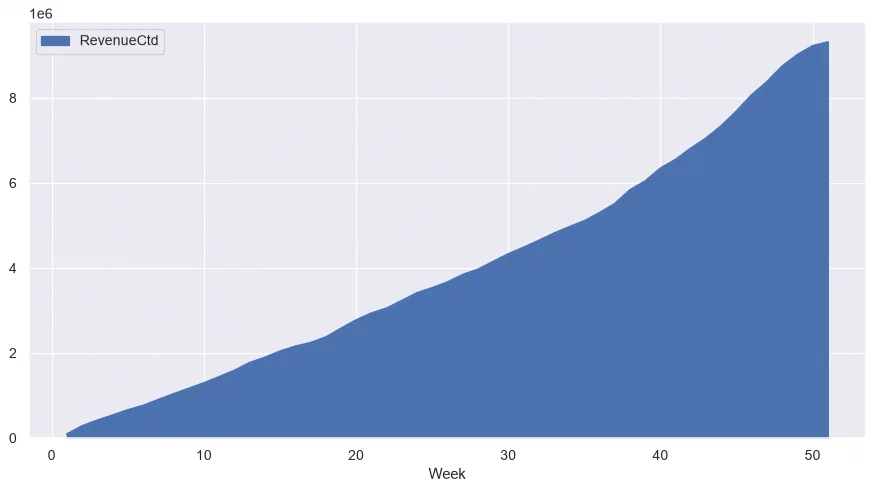
### ✅ 5.8. Add the cumulated revenue in a column named RevenueCtd### Hint: use `cumsum()`df_week['RevenueCtd']=df_week['Revenue'].cumsum()df_week.head()
Week
InvoiceNo
CustomerID
Quantity
Revenue
UnitPrice
RevenueCtd
0
1
320
236
73491
93720.93
1.28
93720.93
1
2
343
235
85626
190994.96
2.23
284715.89
2
3
297
214
67969
133782.91
1.97
418498.80
3
4
431
274
69312
119136.81
1.72
537635.61
4
5
384
270
67613
123642.18
1.83
661277.79
### ✅ 5.9. Plot the weekly cumulated revenue in an area plot### Hint: use `plot.area()`df_week.plot.area(x='Week',y='RevenueCtd')
### ✅ 5.13. Let's group by customers now: number of Orders, Revenue and first date of Order### Hint: use `min()` to get the first date df_clients=(df.groupby('CustomerID').agg({'InvoiceNo':'nunique','Revenue':'sum','InvoiceDay':'min'}))df_clients.head()
CustomerID
InvoiceNo
Revenue
InvoiceDay
12346.0
2
0.00
2011-01-18
12347.0
6
4085.18
2010-12-07
12348.0
4
1797.24
2010-12-16
12349.0
1
1757.55
2011-11-21
12350.0
1
334.40
2011-02-02
### ✅ 5.14. Who are the top 5 biggest spenders ?df_clients.sort_values('Revenue',ascending=False).head()
CustomerID
InvoiceNo
Revenue
InvoiceDay
14646.0
74
267761.00
2010-12-20
18102.0
59
244952.95
2010-12-07
17450.0
54
185919.77
2010-12-07
14911.0
238
125596.25
2010-12-01
12415.0
26
123725.45
2011-01-06
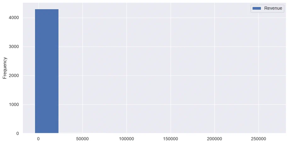
### ✅ 5.15. Plot the Revenue distribution of clients in a histogramdf_clients.plot.hist(y='Revenue')
### ✅ 5.16. Look at the quartiles of Revenue and save it to `df_clients_quantiles`### Hint: use `quantiles([0, .25, .5, .75, .9, .95])`df_clients_quantiles=df_clients['Revenue'].quantile([0,.25,.5,.75,.9,.95])df_clients_quantiles
Revenue
0.0
-4287.63
0.25
289.87
0.5
634.95
0.75
1549.50
0.9
3375.23
0.95
5456.90
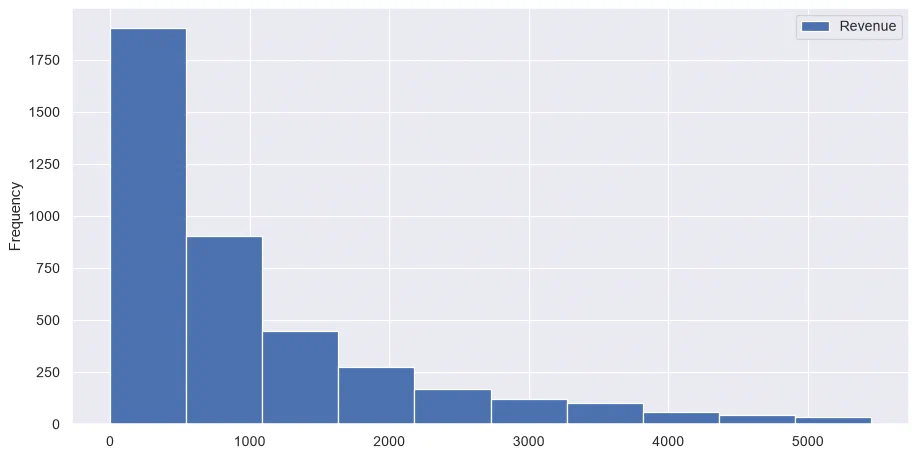
### ✅ 5.17. Now filter client Revenue to be >0 and less than the 95% percentile### And plot the histogram again(df_clients.loc[df_clients['Revenue']>0].loc[df_clients['Revenue']<=df_clients_quantiles[0.95]].plot.hist(y='Revenue'))