#Regression Discontinuity
Introduction
Regression discontinuity is a quasi-experimental design that estimates the causal effect of a treatment by comparing observations just above and below a threshold or cutoff point. It can be used when treatment assignment is determined by a clear cutoff value of a continuous variable, allowing for the estimation of treatment effects in non-randomized setting.
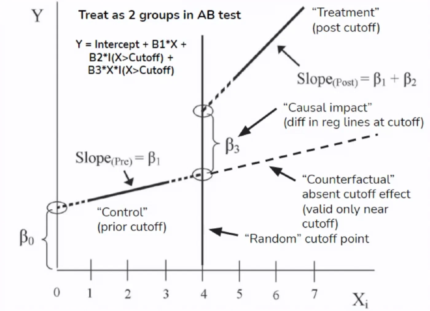
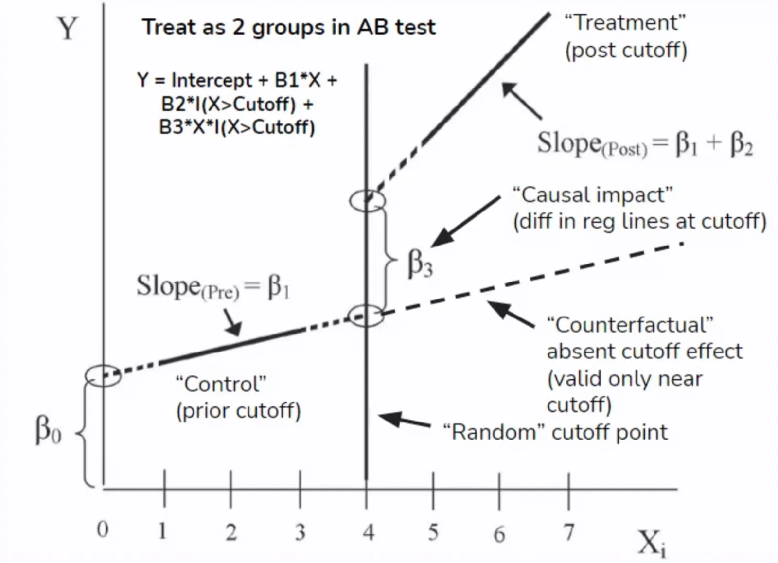
To perform a regression discontinuity analysis, we fit a regression model that includes:
- The running variable X
- A binary indicator for being above or below the threshold
- And an interaction term between the running variable and the binary indicator.
By examining the coefficients and their statistical significance, we can determine if there is a discontinuity in the outcome variable at the threshold, which would suggest a causal effect of the treatment.
Implementation in Python
- First, let’s generate random data, with different intercept and slopes at the threshold:
# Import libraries
import pandas as pd
import numpy as np
import matplotlib.pyplot as plt
import seaborn as sns
import statsmodels.formula.api as smf

# Generate sample data, with discontinuity at a threshold
np.random.seed(42)
df = pd.DataFrame({'x': np.sort(np.random.rand(100))})
threshold = 0.6
df['y'] = np.where(
    df['x'] < threshold,
    2 + 2 * df['x'] + 0.4 * np.random.randn(100),
    2 + 4 * df['x'] + 0.4 * np.random.randn(100)
)
df['treat'] = df['x'] >= threshold

# Plot the data
sns.scatterplot(df, x='x', y='y', hue='treat')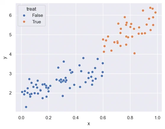
- Now we fit a linear regression with the above mentioned parameters:
# Fit a regression model
model = smf.ols('y ~ x + treat + x:treat', data=df).fit()

# Plot the model results
print(model.summary())
OLS Regression Results
=========================================================================
Dep. Variable: y R-squared: 0.917
Model: OLS Adj. R-squared: 0.914
Method: Least Squares F-statistic: 352.9
Date: Fri, 24 May 2024 Prob (F-statistic): 1.07e-51
Time: 11:14:19 Log-Likelihood: -50.120
No. Observations: 100 AIC: 108.2
Df Residuals: 96 BIC: 118.7
Df Model: 3
Covariance Type: nonrobust
=========================================================================
coef std err t P>|t| [0.025 0.975]
-------------------------------------------------------------------------
Intercept 1.9552 0.096 20.382 0.000 1.765 2.146
treat[T.True] 0.2672 0.482 0.554 0.581 -0.690 1.224
x 2.0988 0.292 7.185 0.000 1.519 2.679
x:treat[T.True] 1.5849 0.655 2.421 0.017 0.285 2.884
=========================================================================
Omnibus: 0.682 Durbin-Watson: 2.213
Prob(Omnibus): 0.711 Jarque-Bera (JB): 0.278
Skew: 0.059 Prob(JB): 0.870
Kurtosis: 3.230 Cond. No. 25.1
=========================================================================The results indicate that:
Intercept: the Intercept below the threshold has an expected value of 1.9552, which is close to the value of 2 that has been set for the simulation data.treat[T.True]: this coefficient represents the difference in the intercept between observations above and below the threshold. Here the coefficient is not statistically significant (p-value = 0.581).x: this coefficient represents the slope of the regression line for observations below the threshold. The coefficient is 2.0988 (close to the slope of 2 that we defined), and it is statistically significant.x:treat[T.True]: this coefficient is the difference in the slope between observations above and below the threshold. The coefficient is statistically significant. This suggests that there is a significant difference in the effect of X on Y between observations above and below the threshold. The slope for observations above the threshold is approximately 2.5849 units higher than the slope for observations below the threshold.
- Plot the fitted regressions over the observed data
# Plot fitted regression
df['y_pred'] = model.predict(df)
sns.scatterplot(df, x='x', y='y', hue='treat', alpha=.6)
sns.lineplot(df, x='x', y='y_pred', hue='treat')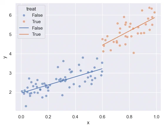
In this case, we can conclude that there is a significant difference in the slope before and after the threshold, meaning that the treatment has an effect.