Reduce required sample size with CUPED

Introduction

When conducting an statistical experiment, there are three levers to reach the necessary statistical power:

↗️ Increase effect size

↗️ Increase sample size

↘️ Decrease variance

Usually, the minimum detectable effect size and the variance are fixed, and we have to play with the sample size to reach the desired statistical power. However, this can be difficult or long to achieve for some experiments.

CUPED is a simple and effective methodology, developed by Microsoft in 2013, and now widely used in the industry, with big Tech companies such as Microsoft, Netflix, BBC, Booking.com, etc.

The original paper claims to have reduced the variance by half on Bing experiments, hence dividing the necessary sample size by approximately two.

There are two methods for implementing CUPED: stratification and covariate-based.

Stratification involves the use of categorical pre-experiment data like country or browser type. We will focus on the other method, the covariate, which uses any continuous metric calculated for each unit before they are exposed to the experiment.

Applying CUPED

Get the data for the metric before the experiment

In theory, you could use any strongly correlated metric, but in practice it is more convenient to use the same metric before the experiment, if available.

Finding the ideal duration for the pre-experiment period is subject to debate. A shorter window doesn’t capture enough variance and a longer window captures noise. For longer experiments, a longer pre-experiment window is needed to ensure that the same users are observed both during and prior to the experiment.

With this pre-experiment metric, calculate a coefficient $\theta$ based on the covariance between values before ( $X$ ) and during ( $Y$ ) the experiment:

\theta = \frac{cov(Y,X)}{var(X)}

For each experiment observation, calculate the adjusted value $\hat{Y}_i$ such as:

\hat{Y}_i = Y_i - \theta X_i

Each observation can for instance be a user, a device, a cookie, etc.

Apply the statistical test between control and treatment groups on the new adjusted values.

The CUPED-adjusted variance should be lower than the raw variance, hence should generate more significant results for the same sample size and effect size.

More precisely, the expected reduction in variance can be calculated with:

var(\hat{Y}) = var(Y-\theta X) = var(Y)(1- corr(X,Y)^2)

Python implementation

Below is an example of Python implementation on synthetic data, that displays a drastic reduction in variance.

We start by generating synthetic data, with a control and target group. Post-experiment, the target group will have an average uplift of +3.

# Load libraries
import numpy as np
import scipy.stats as st
import matplotlib.pyplot as plt
import seaborn as sns

# Generate pre-experiment data 
# for control (x_c) and treatment (x_t) groups
x_c = list(np.random.normal(loc=100, scale=50, size=1000))
x_t = list(np.random.normal(loc=100, scale=50, size=1000))

# Generate post-experiment data 
# for control (y_c) and treatment (y_t) groups
eps_sigma = 40
treatment_lift = 3
y_c = [i + np.random.normal(loc=0, scale=eps_sigma) for i in x_c]
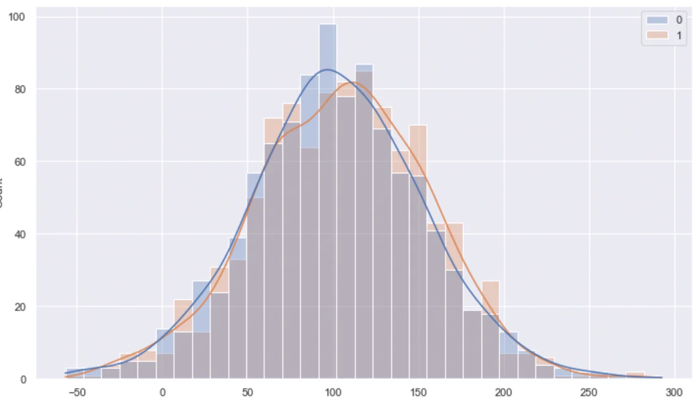
y_t = [i + np.random.normal(loc=0, scale=eps_sigma) + treatment_lift for i in x_t]

We can plot the distributions of each group on the post-experiment phase. Visually, there is no hint of a significant difference between distributions.

# Plot raw distributions
sns.histplot([y_c, y_t], kde=True, alpha=0.3)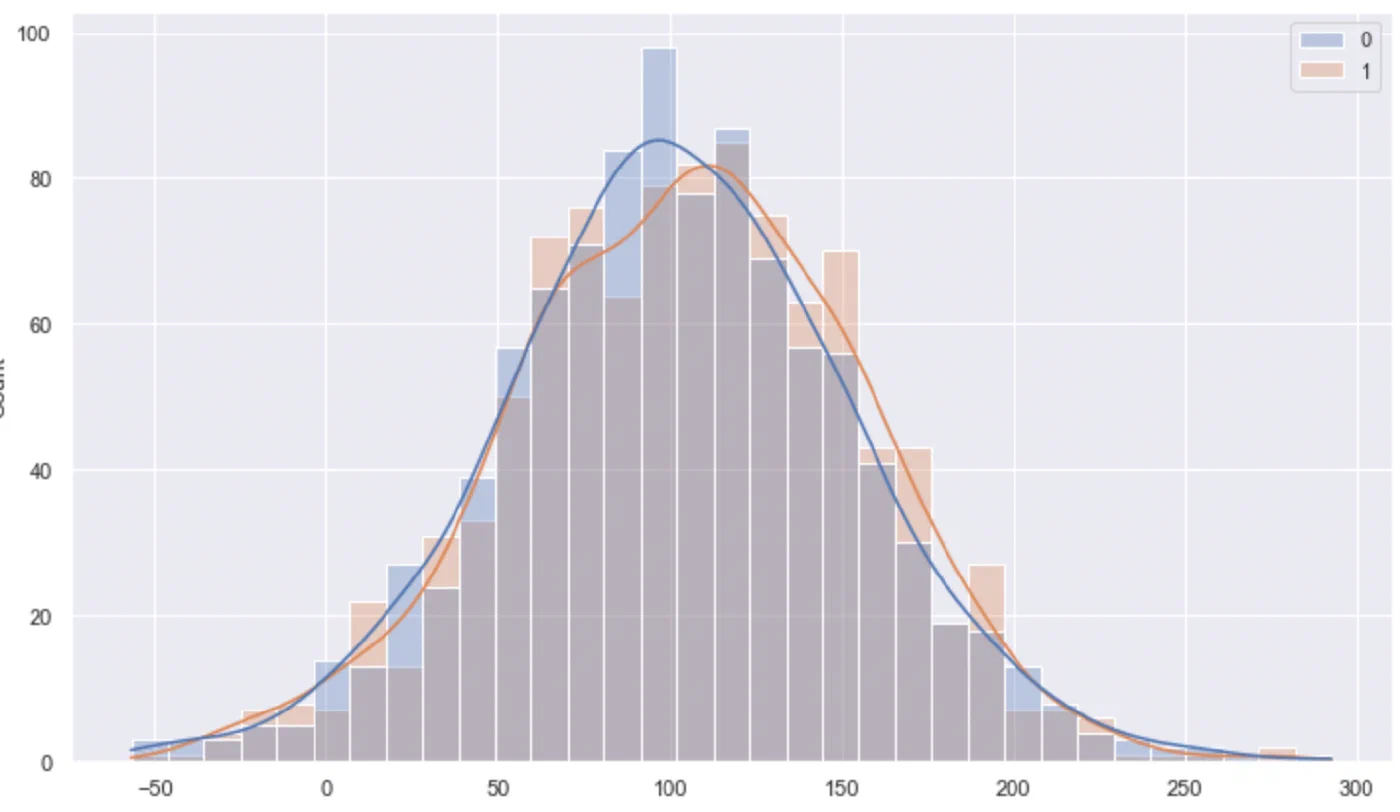

Distribution of control and treatment groups, before CUPED adjustment

We can try to apply a t-test on unadjusted data. We get a non-significant difference, with a p-value around 0.19. The variance of the groups is >2500.

# Show tests results before CUPED
print("Non-adjusted p-value: {:.3f}".format(st.ttest_ind(y_c, y_t)[1]))
print("Non-adjusted lift: {:.3f}".format(np.mean(y_t) - np.mean(y_c)))
print("Non-adjusted variance (control group): {:.0f}".format(np.var(y_c)))
print("Non-adjusted variance (treatment group): {:.0f}".format(np.var(y_t)))

Non-adjusted p-value: 0.194
Non-adjusted lift: 2.948
Non-adjusted variance (control group): 2589
Non-adjusted variance (treatment group): 2553

Now we apply the CUPED formula and compute the adjusted values for each observation. CUPED coefficient θ is around 1.

# Compute CUPED ajusted values
theta = np.cov([y_c+y_t, x_c+x_t])[0,1]/np.var(x_c+x_t)
y_c_adj = [y - x * theta for x, y in zip(x_c, y_c)]
y_t_adj = [y - x * theta for x, y in zip(x_t, y_t)]

print("Theta: {:.3f}".format(theta))

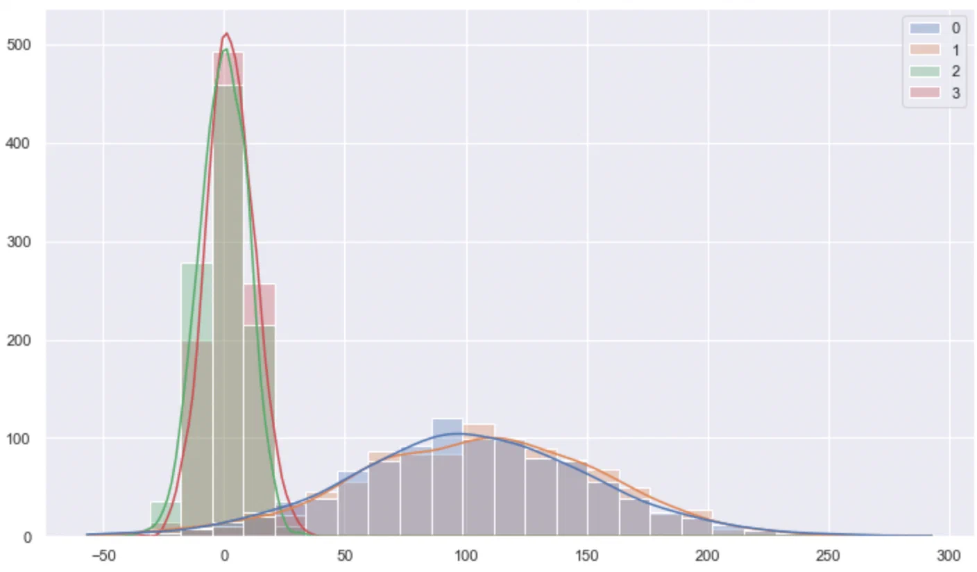
Theta: 1.002

We can plot the distributions before and after CUPED adjustments. It’s visually obvious that the variance had been strongly reduced by CUPED.

# Plot CUPED adjusted distributions
sns.histplot([y_c, y_t, y_c_adj, y_t_adj], kde=True, alpha=0.3)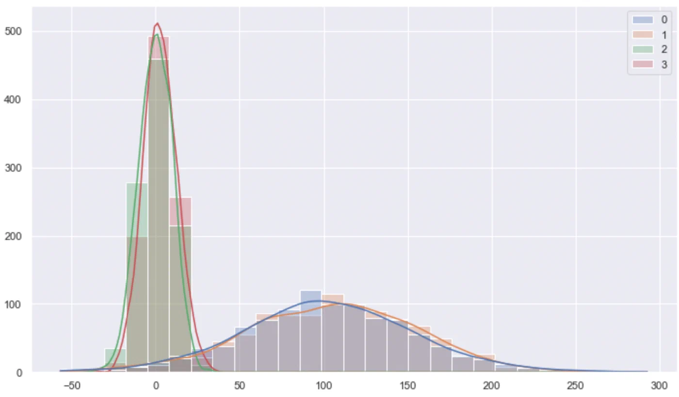

Distribution of control and treatment groups, before and after CUPED adjustment

Finally, we re-apply a t-test on adjusted data. This time, the p-value is 0, thanks to a strong reduction in variance, from around 2500 to 98.

# Show tests results for CUPED-adjusted values
print("CUPED adjusted p-value: {:.4f}".format(st.ttest_ind(y_c_adj, y_t_adj)[1]))
print("CUPED adjusted lift: {:.2f}".format(np.mean(y_t_adj) - np.mean(y_c_adj)))
print("CUPED adjusted variance (control group): {:.0f}".format(np.var(y_c_adj)))
print("CUPED adjusted variance (treatment group): {:.0f}".format(np.var(y_t_adj)))

CUPED adjusted p-value: 0.0000
CUPED adjusted lift: 2.83
CUPED adjusted variance (control group): 98
CUPED adjusted variance (treatment group): 98

##Introduction

##Applying CUPED

##Python implementation

Introduction

Applying CUPED

Python implementation