#PCA vs t-SNE on Fashion-MNIST
Introduction
When a dataset has hundreds of columns, the first thing I want is to see it: are there groups, do the labels separate, which classes overlap? That means bringing it down to two dimensions, and the two methods I reach for are:
- PCA (principal component analysis): a linear projection onto the directions where the data varies the most. Fast, deterministic, and its axes have a meaning.
- t-SNE (t-distributed stochastic neighbor embedding): a non-linear method that tries to keep close points close. Slower, and its axes mean nothing, but it is much better at revealing groups.
To compare them, I used Fashion-MNIST, a set of 70,000 grayscale images of clothes published by Zalando as a harder replacement for the handwritten digits of MNIST. Each image is 28 × 28 pixels, so 784 columns, and belongs to one of 10 classes. The approach follows a Datacamp tutorial.
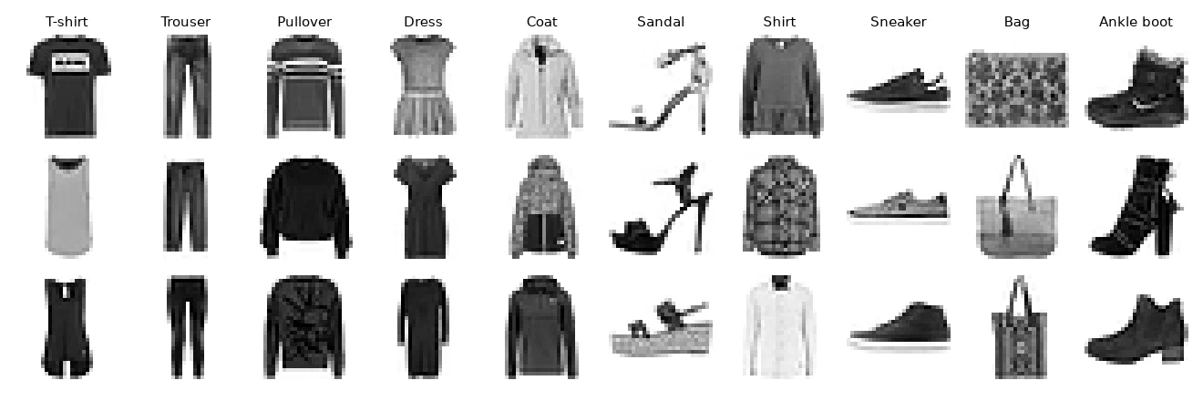
Load the data
The files come in the same binary format as MNIST: a short header, then one byte per pixel.
import gzip
import numpy as np

def load_mnist(path, kind='train'):
    with gzip.open(f'{path}/{kind}-labels-idx1-ubyte.gz') as f:
        labels = np.frombuffer(f.read(), dtype=np.uint8, offset=8)
    with gzip.open(f'{path}/{kind}-images-idx3-ubyte.gz') as f:
        images = np.frombuffer(f.read(), dtype=np.uint8, offset=16).reshape(len(labels), 784)
    return images, labels

X, y = load_mnist('./data', kind='train')

# Keep the first 20,000 images (about 2,000 per class), pixels scaled to [0, 1]
X, y = X[:20000] / 255, y[:20000]PCA
from sklearn.decomposition import PCA

pca = PCA(n_components=50, random_state=123)
X_pca = pca.fit_transform(X)

print(pca.explained_variance_ratio_[:4])
[0.29 0.178 0.06 0.05 ]The first component alone carries 29% of the variance, the first two 47%, and the first 50 components 86%. So two dimensions keep about half the information: enough for a first look, not enough to separate everything.
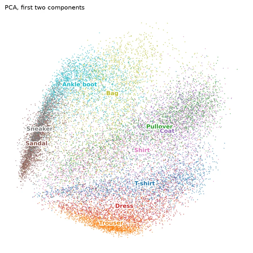
The plot shows a continuum rather than groups. The first component roughly opposes footwear (sandals, sneakers, boots on the left) to clothes, and the second opposes tops to trousers and dresses. Trousers and footwear stand out, but pullovers, coats and shirts are piled on top of each other.
t-SNE
from sklearn.manifold import TSNE

X_tsne = TSNE(random_state=123, init='pca').fit_transform(X)
t-SNE starts from the distances between every pair of points in the original space and looks for a layout in two dimensions where the neighbors stay neighbors. It doesn't care about large distances, only about who is close to whom.
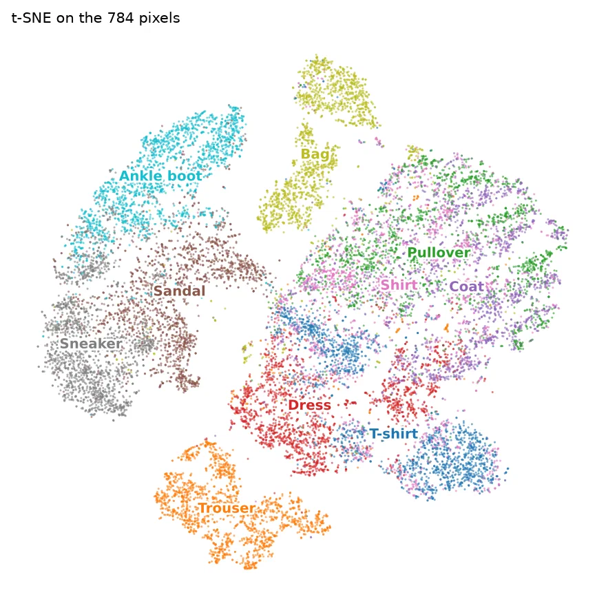
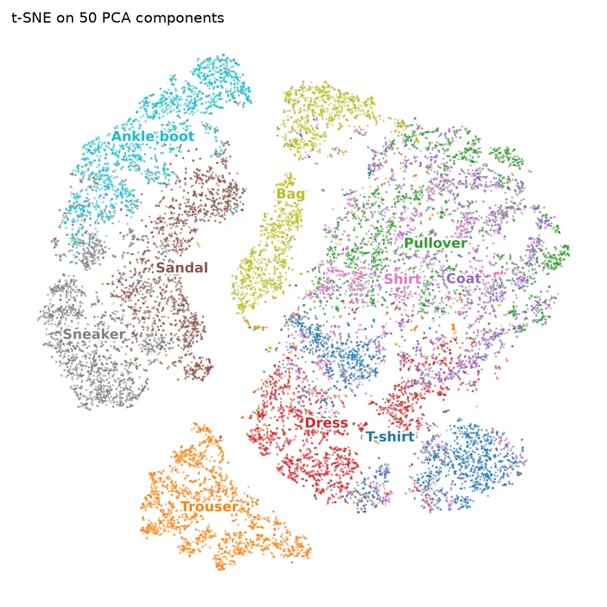
The result is far more readable: trousers, bags, and the three kinds of footwear form their own islands. Sandals sit between sneakers and ankle boots, which makes sense visually. T-shirts and dresses each split into two groups, probably different cuts (with or without sleeves). The large mixed blob of pullovers, coats and shirts remains: these classes simply look alike at 28 × 28 pixels, and a classifier trained on this data makes most of its mistakes there.
The right-hand plot shows a common trick: running t-SNE on the first 50 PCA components rather than on the raw pixels. The layout is almost the same, since those 50 components keep 86% of the variance and drop mostly noise, and on larger datasets it saves a lot of computing time.
Which one to use
| PCA | t-SNE | |
|---|---|---|
| Speed | Instant | Several hundred times slower here; grows quickly with the number of rows |
| Result | Deterministic | Changes with the random seed and the perplexity parameter |
| Axes | Meaningful (combinations of the original columns) | Meaningless |
| Distances | Preserved globally | Only local: the gap between two islands means nothing |
| New data | Can be projected with transform() | No: the whole embedding has to be recomputed |
In practice I use both, one after the other: PCA to reduce the data and understand the main axes of variation, then t-SNE on the PCA output to look for groups. And I keep in mind that the size of a t-SNE island and the distance between islands should not be read: only the fact that points end up together.