Interrupted Time Series

Introduction

Interrupted Time Series is a quasi-experimental design that aims at estimating the causal impact of an intervention at a certain time. The principle is to analyze the time series data collected at multiple intervals before and after the intervention to detect any significant changes in the level and trend of the outcome variable.

This method helps in distinguishing the effect of the intervention from underlying trends and seasonal patterns. By comparing the pre- and post-intervention segments, we can infer whether observed changes can be attributed to the intervention rather than to other external factors.

Formula

In Interrupted Time Series, we typically use segmented (piecewise) regression to model the outcome variable $Y_t$ as a function of time $t$ and the Intervention.

Consider the following segmented regression model:

$Y_t = \beta_0 + \beta_1 \cdot t + \beta_2 \cdot D_t + \beta_3 \cdot (t - T) \cdot D_t + \epsilon_t$

where:

$Y_t$ is the outcome variable at time t.
$t$ is the time variable.
$D_t$ is a dummy variable that takes the value 0 before the intervention and 1 after the intervention.
$T$ is the time point at which the intervention occurs.
$\epsilon_t$ is the error term at time $t$ .

The coefficients should be interpreted as:

Intercept $\beta_0$ : baseline level of the outcome variable at $t=0$ .
Pre-intervention trend $\beta_1$ : slope of the outcome variable before the intervention.
Immediate level change $\beta_2$ : difference in level right after the intervention.
Change in trend $\beta_3$ : change in the slope of the outcome variable after the intervention.

Implementation in Python

Let’s first generate some simulation data, with a change in slope and intercept at intervention time t=50:

# Import libraries
import pandas as pd
import numpy as np
import matplotlib.pyplot as plt
import seaborn as sns
import statsmodels.api as sm

# Simulate pre- and post-intervention data
n_pre, n_post = 50, 50
time = np.arange(n_pre + n_post)
intervention_effect = 20  # Level change due to intervention

data_pre = 0.5 * time[:n_pre] + np.random.normal(loc=0, scale=2, size=n_pre)
data_post = 0.7 * np.arange(n_post) + intervention_effect + np.random.normal(loc=0, scale=2, size=n_post)

# Combine data
df = pd.DataFrame({'time': time, 'data': np.concatenate([data_pre, data_post])})
df['intervention'] = (df['time'] > n_pre).astype(int)

# Plot data
sns.regplot(df.loc[df['intervention'] == 0], x='time', y='data')
sns.regplot(df.loc[df['intervention'] == 1], x='time', y='data')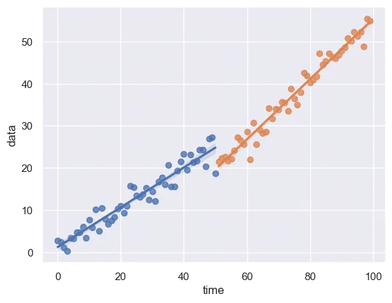

We can now fit a regression and analyse the output:

# Segmented regression analysis
df['time_post'] = df['time'] - n_pre
df['time_post'] = df['time_post'].clip(lower=0)

# Adding constant and trend terms for regression
X = df[['time', 'intervention', 'time_post']]
X = sm.add_constant(X)
y = df['data']

# Fit the model
model = sm.OLS(y, X).fit()
print(model.summary())

                            OLS Regression Results                            
==============================================================================
Dep. Variable:                   data   R-squared:                       0.983
Model:                            OLS   Adj. R-squared:                  0.983
Method:                 Least Squares   F-statistic:                     1897.
Date:                Tue, 18 Jun 2024   Prob (F-statistic):           2.76e-85
Time:                        21:49:29   Log-Likelihood:                -208.49
No. Observations:                 100   AIC:                             425.0
Df Residuals:                      96   BIC:                             435.4
Df Model:                           3                                         
Covariance Type:            nonrobust                                         
================================================================================
                   coef    std err          t      P>|t|      [0.025      0.975]
--------------------------------------------------------------------------------
const            0.9507      0.548      1.734      0.086      -0.138       2.039
time             0.4616      0.019     24.429      0.000       0.424       0.499
intervention    -3.3626      0.795     -4.227      0.000      -4.942      -1.784
time_post        0.2123      0.028      7.704      0.000       0.158       0.267
==============================================================================
Omnibus:                        0.279   Durbin-Watson:                   2.107
Prob(Omnibus):                  0.870   Jarque-Bera (JB):                0.299
Skew:                          -0.121   Prob(JB):                        0.861
Kurtosis:                       2.886   Cond. No.                         251.
==============================================================================

Here’s how to interpret the results:

const is the intercept at time 0
time is the slope before the intervention (0.46) which is significant since the p-value is 0.000. It is close to the 0.50 that we set up for the simulation.
intervention is the change in the intercept immediately after intervention, which in this case is decreased by -3.36 (significant again)
time_post is the change in the slope after intervention, meaning it adds 0.21 on top of the previous slope of 0.46. This coefficient of 0.67 is close to the theoretical parameter.

In this example, we can thus conclude that the intervention had a significant effect on both the level and the slope of the trend, which confirms the simulation parameters.

##Introduction

##Formula

##Implementation in Python

Introduction

Formula

Implementation in Python