Frequentist A/B testing cheatsheet

Introduction

Hypothesis testing, or statistical A/B testing, is a method for comparing two groups or treatments to determine if there is a statistically significant difference between them. The goal of A/B testing is to evaluate the effectiveness of a change or intervention.

In this notebook, we will focus on classical frequentist hypothesis testing, but there are other techniques such as the bayesian methods. More specifically, we’ll test for differences between two samples means (continuous metrics) and proportions.

Fundamentals

Common distributions

Some of the most common distributions encountered in hypothesis testing are:

# Setup
import numpy as np
import seaborn as sns
import matplotlib.pyplot as plt
sns.set_style("white")
fig, ax = plt.subplots(1, 4, figsize=(16,3))

# Normal distribution
from scipy.stats import norm
normal_x = np.arange(-5, 5, 0.01)
ax[0].plot(normal_x, norm.pdf(normal_x, 0, 1))
ax[0].set_title("Normal")

# Student-t distribution
from scipy.stats import t
student_x = np.arange(-5, 5, 0.01)
ddof = 2
ax[1].plot(student_x, t.pdf(student_x, ddof))
ax[1].set_title("Student-t")

# Binomial distribution
from scipy.stats import binom
n = 100
p = .5
binom_x = np.arange(n*p-n*p/2, n*p+n*p/2, 1)
ax[2].bar(binom_x, binom.pmf(binom_x, n, p))
ax[2].set_title("Binomial")

# Binomial distribution
from scipy.stats import poisson
poisson_x = np.arange(0, 20, 1)
ax[3].bar(poisson_x, poisson.pmf(poisson_x, mu=3))
plt.gca().spines['top'].set_visible(False)
ax[3].set_title("Poisson")

# Aesthetics
for axe in ax:
    sns.despine(ax=axe)
    axe.set_yticks([])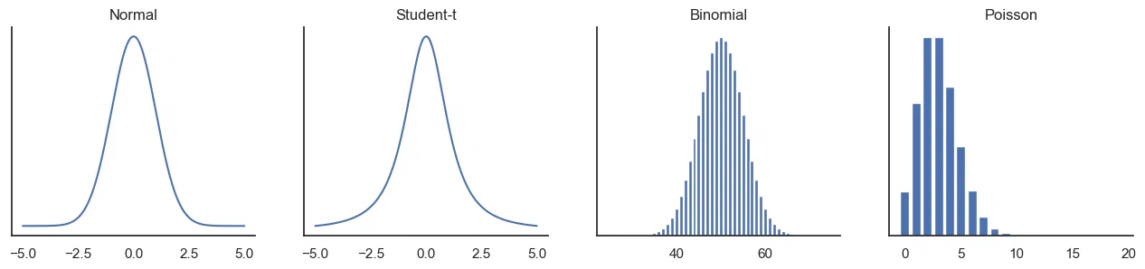

Normal distribution: continuous probability distribution that is symmetric and bell-shaped. It is generally used to model the distribution of sample means for continuous data, when the sample size is large and the population standard deviation is known or can be estimated.
Student’s t-distribution: similar to the normal distribution but has thicker tails, making it more appropriate when the sample size is small (< 30 observations) or the population standard deviation is unknown.
Binomial distribution: discrete probability distribution that is used to model the distribution of binary outcomes, such as clicks, conversions, or success/failure events. For example, it is often used to calculate the difference in conversion rates or click-through rates between two groups.
Poisson distribution: discrete probability distribution that is used to model the distribution of rare events, such as the number of purchases or sign-ups. It is often used in A/B testing to analyze count data, such as the number of conversions or clicks, when the rate of occurrence is low.

Definitions

Here are the most important concepts used in hypothesis testing:

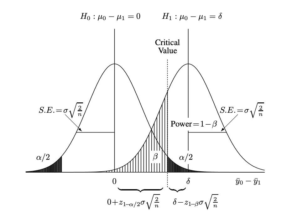
Hypotheses: a hypothesis is a statement about the population being tested. In A/B testing, there are two hypotheses: the null hypothesis $H_0$ and the alternative hypothesis $H_1$ . The null hypothesis usually states that there is no difference between the two groups, while the alternative hypothesis states that there is a difference.
Test statistic: summary statistic that is calculated from the data and is used to determine the likelihood of the null hypothesis being true. It is usually the standardized difference between means or proportions.
P-value: probability of obtaining a test statistic as or more extreme than the observed one, assuming that the null hypothesis is true. It is used to determine whether the null hypothesis should be rejected or not. A p-value less than the significance level $\alpha$ indicates that the results are statistically significant.
Significance level α: probability of rejecting the null hypothesis when it is actually true. It is usually set at 0.05, which means that there is a 5% chance of rejecting the null hypothesis when it is actually true.
Beta value β: probability of failing to reject the null hypothesis when the alternative hypothesis is actually true. In other words, beta represents the likelihood of not detecting a true effect in the sample. It is often set at 20%.
Power (1 − β): probability of rejecting the null hypothesis when it is actually false. It depends on several factors, such as the sample size, effect size, and significance level.
Type I error aka α error: occurs when the null hypothesis is rejected when it is indeed true.
Type II error aka β error: occurs when the null hypothesis is not rejected, whereas it should because there really is a difference.
Sensitivity aka Recall aka True positive rate: measure of the proportion of actual positive cases that are correctly identified as positive.

Here is graphical representation of some of these concepts:

Source: vanbelle.org

Formulas

Here are the most important statistics and their formulas, for both continuous and proportion data:

Statistic	Notation	Formula for continuous data	Formula for proportions
Sample size	$n$	-	-
Sample mean	$x̄$	$\frac{\sum x}{n}$	-
Sample proportion	$\hat p$	-	$k/n$
Sample variance	$s^2$	$\frac{\sum{(x - \bar x)^2}}{n-1}$	$\hat p (1- \hat p)$
Sample standard deviation	$s$	$\sqrt{\frac{\sum{(x - \bar x)^2}}{n-1}}$	$\sqrt{\hat p (1- \hat p)}$
Standard Error of the Mean / of the Proportion	$SEM$ * / * $SEP$	$s/\sqrt n$	$s/\sqrt n$

Typically in A/B tests, we compare the means or proportions between two samples (as opposed to comparing a sample to a general population). Here are the basics to calculate statistical significance:

Test	Distribution	Standard Error (SE)	Test statistic	Confidence Interval of the difference
Difference in samples means	Student-t	$\sqrt{\frac{s^2_1}{n_1}+\frac{s^2_2}{n_2}}$	$\frac{\bar{x}_2 - \bar{x}_1}{SE}$	$(\bar{x_2} - \bar{x_1}) \pm t \cdot SE$
Difference in samples proportions	Binomial	$\sqrt{\frac{\hat p_1 (1-\hat p_1)}{n_1}+\frac{\hat p_2 (1-\hat p_2)}{n_2}}$	$\frac{\hat p_2 - \hat p_1 }{SE}$	$(p̂_2 − p̂_1) ± z \cdot SE$

As a side note, keep in mind that plotting the confidence intervals of each sample mean or proportion does not necessarily reflect the statistical significance of the difference:

It is sometimes claimed that if two independent statistics have overlapping confidence
intervals, then they are not significantly different. This is certainly true if there is
substantial overlap. However, the overlap can be surprisingly large and the means
still significantly different. Confidence intervals associated with statistics can overlap as much as 29% and the statistics can still be significantly different.

– Gerald van Belle, Statistical Rules of Thumb

Implementation in Python

Continuous data

Let’s use the formulas above to test for the statistical difference between two samples means. We’ll first compute the formulas manually, then check our results with SciPy functions out-of-the-box.

Create sample data, with two normally distributed samples, and plot the distributions:

# Import libraries
import numpy as np
import scipy.stats as st
import seaborn as sns
import matplotlib.pyplot as plt

# Create two normally distributed samples
np.random.seed(2)
h1 = np.random.normal(loc=10, scale=2, size=100)
h2 = np.random.normal(loc=10.1, scale=2, size=80)

# Plot distributions
fig, ax = plt.subplots(figsize=(8,4))
sns.histplot(h1, binwidth=1, color='steelblue')
sns.histplot(h2, binwidth=1, color='green')
ax.axvline(np.mean(h1), linestyle='--', color='darkblue')
ax.axvline(np.mean(h2), linestyle='--', color='darkgreen')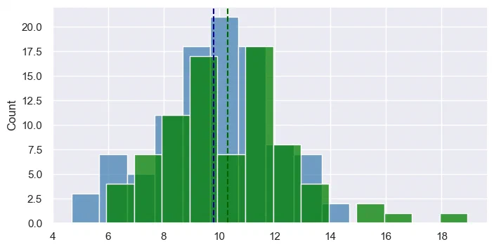

Manually calculate the results, applying the formulas from the previous section:

# Sample sizes
n1 = len(h1); n2 = len(h2)

# Means
x1 = np.mean(h1); x2 = np.mean(h2)

# Standard deviations
s1 = np.std(h1, ddof=1); s2 = np.std(h2, ddof=1)

# t-statistic
t = (x2 - x1) / np.sqrt(s1**2/n1 + s2**2/n2)

# Print results
print("Difference in means: {:.4f}".format(x2 - x1))
print("t-score: {:.4f}".format(t))
print("p-value: {:.4f}".format(st.t.sf(abs(t), df=n1+n2-2) *2))   # Multiply by 2 for two-tailed test

Difference in means: 0.5219
t-score: 1.5606
p-value: 0.1204

With a p-value above 0.05, there is no significant difference with 95% confidence between the means of the groups.

Check the results with SciPy, with a simple one-liner:

# Check results with scipy
t_test = st.ttest_ind(h2, h1, alternative='two-sided', equal_var=False)
print("t-score: {:.4f}\np-value: {:.4f}".format(t_test[0], t_test[1]))

t-score: 1.5606
p-value: 0.1206

As expected, we get the same results than previously.

Proportions

Let’s now calculate in Python a difference in proportions between two groups, just like we did for continous metrics. For that, we will use the Z-test. It would also be possible to use the Chi-squared test.

Generate sample data:

# Import libraries
import numpy as np
import statsmodels.stats.proportion as ssm

# Create two binomial samples
n1 = 1000; n2 = 800
k1 = 150; k2 = 140

# Compute proportions
p1 = k1/n1
p2 = k2/n2
p = (k1+k2)/(n1+n2)

Manually calculate the results, applying the formulas:

# Standard Error of the Proportion
sep = np.sqrt(p*(1-p)*(1/n1+1/n2))

# z-statistic
z = (p2 - p1) / sep

print("z-score: {:.4f}".format(z))
print("p-value: {:.4f}".format(st.norm.sf(abs(z))*2))   # Multiply by 2 for two-tailed test

z-score: 1.4336
p-value: 0.1517

Since the p-value is >0.05, we cannot conclude to a significant difference.

Double-check the results with the StatsModels function:

# Check with statsmodels
prop_z_test = ssm.proportions_ztest(
    count=[k2, k1],
    nobs=[n2, n1],
    alternative='two-sided',
)

print("z-score: {:.4f}\np-value: {:.4f}".format(prop_z_test[0], prop_z_test[1]))

z-score: 1.4336
p-value: 0.1517

And as expected, we get the exact same results.

Resources

Statistics for Dummies cheat sheet
Evan’s calculator for sample size
Statistical Rules of Thumb by Gerald Van Belle

##Introduction

##Fundamentals

###Common distributions

###Definitions

##Formulas

##Implementation in Python

###Continuous data

###Proportions

##Resources