#Difference-in-differences method
Introduction
The difference-in-differences (DiD) method is a quasi-experimental research design that is used to estimate the causal effect of a treatment on an outcome.
The method compares the outcomes of two groups of units: a treatment group that received the treatment and a control group that did not receive the treatment. Then it compares the changes in the outcomes of the two groups over time.
If the treatment group experiences a greater change in the outcome than the control group, then the DiD method can be used to infer that the treatment caused the change in the outcome.
Calculation
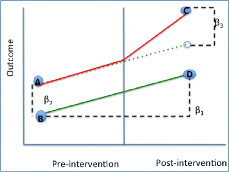
The DiD method assumes that the two groups would have experienced similar changes in the outcome if the treatment had not been implemented. It’s sometimes referred to as “parallel trends assumption”. In other words, the only difference between the two groups should be the treatment.
To assess this difference, a regression can be used, like the following:
When should DiD be used?
The DiD method can be used a substitute when it is not possible to conduct a randomized controlled trial. However, there are two requirements:
- Treatment and control group trends should be highly correlated (parallel) before the treatment is implemented.
- Treatment should be implemented at the same time for all units in the treatment group.
One problem of this method is that, in picking a control group that satisfies the parallel assumption, it can be arbitrary to choose one in particular. To avoid this, a more advanced option is the Synthetic Control* *method, where many control groups can be averaged.
Python implementation
- Let’s start with example data from a website experiment, where each user is randomly assigned to a Control or Target group.
We aggregate data by date, and compute the daily conversion_rate of each group, simply as the number of conversions over number of sessions.
We need a numeric column day rather than a datetime, which is the rank of the day since the beginning of available data, including the pre-experiment period.
We also create binary columns is_target as indicator for the target group, and is_after that indicates the period of the experiment.
# Example data
df_did| day | group | is_target | is_after | sessions | conversions | conversion_rate |
|---|---|---|---|---|---|---|
| 0 | control | 0 | 0 | 584 | 373 | 0.246575 |
| 1 | control | 0 | 0 | 378 | 332 | 0.314815 |
| 2 | control | 0 | 0 | 331 | 290 | 0.280967 |
| 3 | control | 0 | 0 | 445 | 376 | 0.328090 |
| 4 | control | 0 | 0 | 645 | 479 | 0.289922 |
| ... | ... | ... | ... | ... | ... | ... |
| 57 | target | 1 | 1 | 654 | 331 | 0.191131 |
| 58 | target | 1 | 1 | 568 | 364 | 0.285211 |
| 59 | target | 1 | 1 | 763 | 422 | 0.245085 |
| 60 | target | 1 | 1 | 1054 | 537 | 0.245731 |
| 61 | target | 1 | 1 | 1885 | 735 | 0.187798 |
- We can plot the conversion rates of each group before and after the start of the experiment, as well as regression lines for each period and group. This helps us assess the essential assumption that both trends were parallel before the change. Beyond visual inspection, you can fit a regression for each group, and run a statistical test to ensure that there is no significant difference in their slopes for the pre-change period.
# Plot conversion rate by group and period (before/after)
fig, ax = plt.subplots(figsize=(6,8))
sns.lineplot(data=df_did, x='day', y='conversion_rate', hue='group')
sns.regplot(
		data=df_did.loc[lambda x: (x['is_target'] == 0) & (x['is_after'] == 0)],
		x='day', y='conversion_rate', marker='.', color='steelblue')
sns.regplot(
		data=df_did.loc[lambda x: (x['is_target'] == 1) & (x['is_after'] == 0)],
		x='day', y='conversion_rate', marker='.', color='peru')
sns.regplot(
		data=df_did.loc[lambda x: (x['is_target'] == 0) & (x['is_after'] == 1)],
		x='day', y='conversion_rate', marker='.', color='steelblue')
sns.regplot(
		data=df_did.loc[lambda x: (x['is_target'] == 1) & (x['is_after'] == 1)],
		x='day', y='conversion_rate', marker='.', color='peru')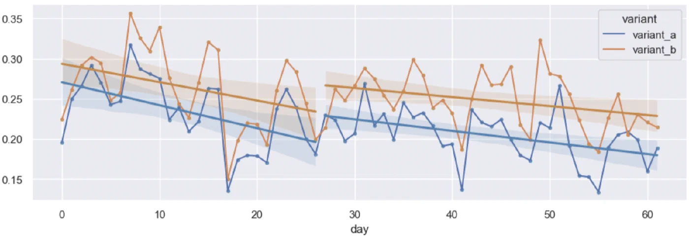
- Finally we apply the actual difference-in-difference test, by fitting a linear regression and looking at the coefficients.
# Import library
import statsmodels.formula.api as smf

# Fit DiD model
did_model = smf.ols(
	'conversion_rate ~ is_target * is_after',
	data=df_did.reset_index()
)
results = did_model.fit()

# Display results
print(results.summary())
OLS Regression Results
================================================================================
Dep. Variable: conversion_rate R-squared: 0.336
Model: OLS Adj. R-squared: 0.320
Method: Least Squares F-statistic: 20.26
Date: Sat, 13 May 2023 Prob (F-statistic): 1.09e-10
Time: 14:50:56 Log-Likelihood: 202.05
No. Observations: 124 AIC: -396.1
Df Residuals: 120 BIC: -384.8
Df Model: 3
Covariance Type: nonrobust
===================================================================================
coef std err t P>|t| [0.025 0.975]
-----------------------------------------------------------------------------------
Intercept 0.2559 0.009 27.578 0.000 0.238 0.274
is_target 0.0289 0.013 2.201 0.030 0.003 0.055
is_after -0.0634 0.012 -5.136 0.000 -0.088 -0.039
is_target:is_after 0.0255 0.017 1.460 0.147 -0.009 0.060
==============================================================================
Omnibus: 3.972 Durbin-Watson: 1.186
Prob(Omnibus): 0.137 Jarque-Bera (JB): 3.736
Skew: -0.425 Prob(JB): 0.154
Kurtosis: 3.016 Cond. No. 7.33
==============================================================================
Notes:
[1] Standard Errors assume that the covariance matrix of the errors is correctly specified.In this case, the p-value is 0.147 and the 95% confidence interval includes 0, so it’s not significant. We cannot conclude that the treatment had an effect.