#Delta Method for A/B testing
Introduction
When running an experiment, sometimes the randomisation unit is different from the analysis unit. In this case, the assumption of independence between each observation may not hold anymore.
Since the independent and identically distributed (i.i.d.) assumption is violated, “the naïve variance calculation will likely underestimate variance, leading to false detection of changes that are actually within normal variation” (source). For this reason, it’s not possible to apply a z-test (or t-test) without adjustement.
Let’s take an example
Imagine you’re running an A/B test for an app, where you want to test a new feature on a subset of users that should increase their conversion rate, i.e. the proportion of sessions that end up in a conversion.
You start by selecting at random two groups of users, for Control and Target. Then you roll out your new feature to users in the target group. And you want to measure the effect on the conversion rate.
However, the probabilities that visits end up in a conversion for user are not independent, they are clearly correlated. Users have different behaviours, and some users have a consistently higher or lower conversion rate than others.
Note that, the higher the number of observations per randomisation unit (e.g. sessions per user), the more distortion in variance there is. In our example, the difference in variance is far worse if the experiment runs for two months, during which users may generate 30 sessions, rather than one week, where they will have ~3 sessions.
Formula and implementation
The Delta method estimates the true variance based on the Central Limit Theorem and using a Taylor expansion. The full formula is the following:
In Python, this can be written as:
import numpy as np
delta_variance = \
    (np.var(X, ddof=1) / np.mean(Y)**2 + \
    np.var(Y, ddof=1)*(np.mean(X)**2 / np.mean(Y)**4) - \
    2*np.cov(X, Y, ddof=1)[0][1]*(np.mean(X)/np.mean(Y)**3)) / len(Y)
where X and Y are lists (or any kind of iterable like pd.Series):
Xis the ratio nominator, e.g. number of conversions per userYis the ratio denominator, e.g. number of sessions per user
Implementing our example
There are 3 simple steps, provided that you have the data in the correct format.
- As experiment data, we have a DataFrame of users that were randomly assigned to the Control or Target. We recorded their session in the app, and the number of sessions that generated a conversion.
The table contains one row per user, with their group, total number of sessions, total number of conversions, and conversion_rate calculated as conversions over sessions:
| group   | user_id          | sessions | conversions | conversion_rate |
|:--------|:-----------------|---------:|------------:|----------------:|
| Control | b0cc6b25669f1cfb |      150 |          62 |        0.413333 |
| Target  | 1cc2f0c081cff495 |       20 |          11 |        0.550000 |
| Control | 0dfa929aa7cea87a |       31 |           6 |        0.193548 |
| Target  | 0dfa929aa7cea87a |       39 |           9 |        0.230769 |
| Control | e1916d7a661d210f |        3 |           2 |        0.666667 |
We check the summary statistics for each group:
# Summary stats
(
    df
    .groupby(['group'])
    .agg({'user_id': 'count', 'sessions': 'sum', 'conversions': 'sum'})
    .assign(conversion_rate=lambda x: (x['conversions']/x['sessions']).round(3))
)| group | users | sessions | conversions | conversion_rate |
|---|---|---|---|---|
| Control | 488 | 37689 | 7662 | 0.2032 |
| Target | 493 | 45106 | 8134 | 0.1803 |
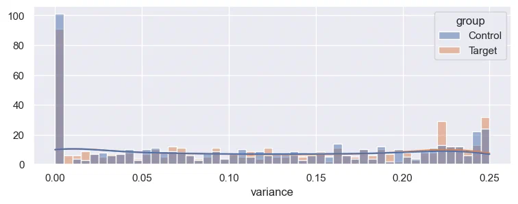
And we can plot the distributions of the variances:
# Plot distributions
import seaborn as sns
import matplotlib.pyplot as plt
sns.histplot(
    df.assign(variance=lambda x: x['conversion_rate'] * (1-x['conversion_rate'])),
    x='variance', hue='group', bins=50, kde=True
)
- We now calculate the Delta-estimated variances for control and target groups.
First we write the function:
# Function to get the Delta adjusted variance of the ratio X/Y
def delta_var(x, y):
    mean_x = np.mean(x)
    mean_y = np.mean(y)
    var_x = np.var(x, ddof=1)
    var_y = np.var(y, ddof=1)

    cov_xy = np.cov(x,y,ddof=1)[0][1]
    delta_variance = \
        (var_x/mean_y**2 + var_y*(mean_x**2/mean_y**4) - \
        2*cov_xy*(mean_x/mean_y**3)) / len(y)

    return delta_variance
Then we apply the function to each group, and get the estimated variances:
# Compute estimated variances
var_delta_c = delta_var(
    x=df.loc['Control', 'conversions'],
    y=df.loc['Control', 'sessions']
)

var_delta_t = delta_var(
    x=df.loc['Target', 'conversions'],
    y=df.loc['Target', 'sessions']
)- We can finally apply a usual z-test or t-test with the adjusted variances:
# Compute z-test
from scipy import stats

mean_c = df.loc['Control', 'conversions'].sum() / df.loc['Control', 'sessions'].sum()
mean_t = df.loc['Target', 'conversions'].sum() / df.loc['Target', 'sessions'].sum()
mean_diff = mean_t - mean_c
var_delta = var_delta_c + var_delta_t
delta_z_score = mean_diff / np.sqrt(var_delta)
delta_p_value = stats.norm.sf(abs(delta_z_score)) * 2

pd.DataFrame({
    'Control mean': mean_c.round(3),
    'Target mean': mean_t.round(3),
    'Difference': mean_diff.round(3),
    'Control variance': var_delta_c,
    'Target variance': var_delta_t,
    'z-score': delta_z_score.round(4),
    'p-value': delta_p_value.round(4),
}, index=['value']).transpose()| Value | |
|---|---|
| Control mean | 0.203 |
| Target mean | 0.180 |
| Difference | -0.023 |
| Control variance | 0.000167 |
| Target variance | 0.000146 |
| z-score | -1.298 |
| p-value | 0.1943 |
The p-value is 0.19 and cannot be considered significant with 95% confidence.
Sample size estimation
See also: Calculate the sample size for A/B testing