#Calculate confidence intervals in Python
Introduction
Confidence intervals (CI) are a way of estimating a population parameter (e.g., mean, variance) from a sample of data. They provide a range of values within which the true population parameter is likely to fall, with a certain level of confidence. For example, a 95% confidence interval means that we can be 95% confident that the true population parameter lies within the specified range.
The confidence interval formula is:
where:
- * *is the sample mean, or sample for probabilities
- t is the t-value from the t-distribution corresponding to the desired confidence level (e.g., 1.96 for a 95% confidence interval)
- s is the sample standard deviation, calculated as:
- for continuous metrics:
- for probabilities:
- is the sample size
Now let’s see how we can simply implement this in Python.
Generate random data
We begin by generating synthetic data, drawing a random sample of size 100 from a normal distribution with mean 40 and standard deviation 10.
# Import libraries
import numpy as np
import pandas as pd

# Generate sample from a normal distribution
np.random.seed(222)
df = pd.DataFrame({'value': np.random.normal(
		loc=40,
		scale=10,
		size=100)
})

# Show sample actual values
df.describe().head(3).round(2)| value | |
|---|---|
| count | 100.00 |
| mean | 40.26 |
| std | 9.15 |
Calculate confidence interval
Since the formula is straightforward, we can easily compute the confidence interval without any additional library:
# Calculate confidence interval
x_bar = df.mean()[0]     # Sample mean
sigma = df.std()[0]      # Standard deviation
n = len(df)              # Sample size
t_score = 1.96           # Approximative t-score for 95% two-sided interval

# Calculate margin of error and confidence interval
moe = t_score * sigma / np.sqrt(n)
ci = [x_bar - moe, x_bar + moe]
ci
[38.46, 42.05]But more conveniently, we can compute it as a one-liner with the scipy package:
# Import library
import scipy.stats as stats

# Calculate 95% confidence interval
stats.t.interval(
    alpha=0.95, df=n-1, loc=x_bar, scale=sigma / np.sqrt(n)
)
[38.44, 42.07]The intervals are almost identical, and the 2nd decimal difference is explained by the fact that we have approximated the t-value to 1.96 in the first “manual” method.
Plot distribution and confidence interval
Finally, let’s plot a histogram of the the sample distribution with the population mean, sample mean, and confidence interval of the sample mean.
# Import libraries
import seaborn as sns
import matplotlib.pyplot as plt

# Plot histogram and true population mean
sns.histplot(df, binwidth=2)
plt.axvline(40, color='darkslateblue')

# Plot sample mean and confidence interval
plt.axvline(x_bar, color='orange', linestyle='--')
plt.axvspan(ci[0], ci[1], alpha=0.3, color='gold');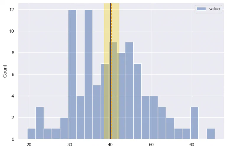
The plot above shows the sample distribution with a population mean of 40, as well as the sample mean 40.26 and a 95% confidence interval of [38.46, 42.05].