Bayesian hypothesis testing

Introduction

In recent years, Bayesian methods for hypothesis testing have become increasingly popular. They are said to be superior than classical frequentist methods in several aspects, including interpretability, incorporation of priors, and resistance to data peeking.

In this post, we will implement basic Bayesian hypothesis testing in Python.

Generate sample data

We begin by generating sample conversion data, in two groups, Control and Treatment.

$n_c$ and $n_t$ are the number of observations in each group (number of sessions, for example)
$k_c$ and $k_t$ are the number of conversions (e.g. number of sessions with a conversion)
$p_c$ and $p_t$ are the observed conversion rates, calculated as $k/n$

# Import libraries
import pandas as pd
import numpy as np
import matplotlib.pyplot as plt
import seaborn as sns
import scipy.stats as st
import scipy.special as sp
sns.set()

# Generate sample conversion data
np.random.seed(42) 
n_c = 1200
n_t = 1000
control_data = np.random.binomial(1, p=0.11, size=n_c)
treatment_data = np.random.binomial(1, p=0.15, size=n_t)
p_c = control_data.sum()/len(control_data)
p_t = treatment_data.sum()/len(treatment_data)
k_c = control_data.sum()
k_t = treatment_data.sum()

print("Control rate: {:.4f}".format(p_c))
print("Treatment rate: {:.4f}".format(p_t))
print("Relative difference: {:+.4f}".format((p_t-p_c)/p_c))

Control rate: 0.1217
Treatment rate: 0.1420
Relative difference: +0.1671

We observe conversion rates of approximately 0.12 for the control group and 0.14 for the target group.

Frequentist test

Let's begin with a classical t-test to initially assess the significance of the difference between groups.

# Frequentist t-test, for reference
ttest = st.ttest_ind(control_data, treatment_data, equal_var=False)
print("t-statistic: {:.4f}".format(ttest[0]))
print("p-value: {:.4f}".format(ttest[1]))

t-statistic: -1.3995
p-value: 0.1618

In this case, the p-value exceeds 0.05. Thus, there is no significant difference at a confidence level of 95%.

Define prior parameters

Defining the right prior parameters is a matter of debate. They should incorporate prior knowledge of the data. In the code below, we could use pre-experiment data of a period similar to the experimentation period length, and use it as follows:

n_prior: number of observations in the pre-experiment period
k_prior: number of conversions in the pre-experiment period

In this example however, we’ll greatly simplify by setting alpha and beta to 1.

# Prior parameters
k_prior = 0
n_prior = 0

alpha_prior = 1 + k_prior
beta_prior = 1 + n_prior - k_prior

control_alpha_prior = alpha_prior
control_beta_prior = beta_prior

treatment_alpha_prior = alpha_prior
treatment_beta_prior = beta_prior

Conjugate distributions

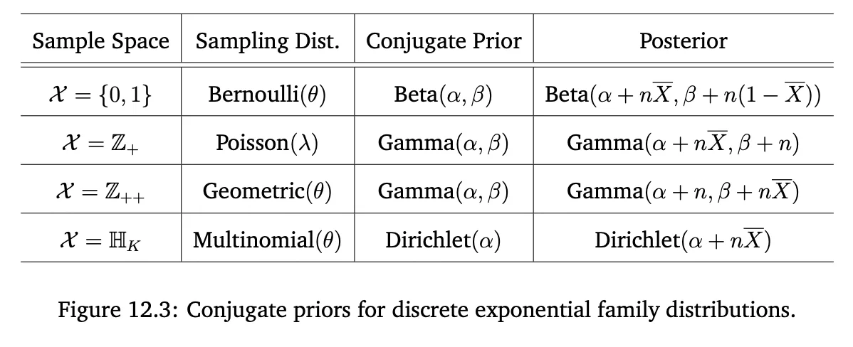
In our case, the prior and posterior functions are conjugate, meaning they belong to the same family. This allows us to compute the posterior analytically rather than through simulation.

Source

Assess statistical difference

Let’s calculate and plot the posterior distributions, based on the observed data.

# Calculate posterior parameters
control_alpha_posterior = control_alpha_prior + k_c
control_beta_posterior = control_beta_prior + n_c - k_c

treatment_alpha_posterior = treatment_alpha_prior + k_t
treatment_beta_posterior = treatment_beta_prior + n_t - k_t

# Create Beta distributions for the posterior
control_posterior = st.beta(control_alpha_posterior, control_beta_posterior)
treatment_posterior = st.beta(treatment_alpha_posterior, treatment_beta_posterior)

# Plot posterior distributions
x = np.linspace(.05, .2, 1000)
control_pdf = control_posterior.pdf(x)
treatment_pdf = treatment_posterior.pdf(x)

fig, ax = plt.subplots(figsize=(6,3))
sns.lineplot(x=x, y=control_pdf)
sns.lineplot(x=x, y=treatment_pdf)
ax.set_title("Posterior distributions")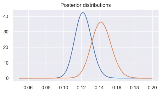

We can visually see the difference between the Control (~0.12) and Target (~0.14) groups. Now we want to assess for the statistical significance of this difference.

Checking fit of posterior functions

To make sure that our posterior functions approximately fit the observed data, we can plot the observed data against simulated samples.

# Visually check fit of posterior functions
control_samples = control_posterior.rvs(10000)
treatment_samples = treatment_posterior.rvs(10000)
control_simulated_data = np.random.binomial(n=n_c, p=control_samples)
treatment_simulated_data = np.random.binomial(n=n_t, p=treatment_samples)

fig, ax = plt.subplots(1, 2, figsize=(10,4))
sns.histplot(control_simulated_data, kde=False, binwidth=1, color='steelblue', alpha=.3, ax=ax[0])
sns.histplot(treatment_simulated_data, kde=False, binwidth=1, color='darkorange', alpha=.3, ax=ax[1])
ax[0].axvline(k_c, color='steelblue', linestyle='dashed', linewidth=2)
ax[1].axvline(k_t, color='darkorange', linestyle='dashed', linewidth=2)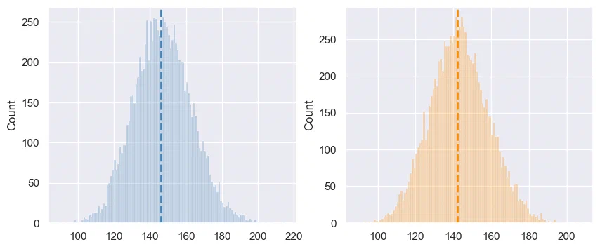

Visually, the samples are distributed around the means of each group, which is a good indication that our posterior models are correct.

Probability A beats B

We can now compute the probability that Treatment group is greater than Control group, in two different ways.

A first method is to sample the data, and see how many times Treatment beats Control. We can re-use the samples that were generated above, for checking the fit of posterior distributions.

# Calculate the proportion of times Treatment group outperforms Control group
prob_treatment_greater = (treatment_samples > control_samples).mean()
print("Probability that Treatment > Control (sampling): {:.3f}".format(prob_treatment_greater))

Probability that Treatment > Control (sampling): 0.921

We can also compute it analytically:

def probability_B_beats_A(alpha_A, beta_A, alpha_B, beta_B):
    total = 0.0
    for i in range(0,alpha_B-1):
        total += np.exp(sp.betaln(alpha_A+i, beta_B+beta_A)
            - np.log(beta_B+i) - sp.betaln(1+i, beta_B) - sp.betaln(alpha_A, beta_A))
    return total

print("Probability that Treatment > Control (analytical): {:.3f}".format(probability_B_beats_A(control_alpha_posterior, control_beta_posterior, treatment_alpha_posterior, treatment_beta_posterior)))

Probability that Treatment > Control (analytical): 0.912

As expected, we get similar results between the two methods.

Credible Interval

We can also calculate the 95% Credible Interval, which is similar to the Confidence Interval used in frequentist tests, to determine the difference between groups.

diff_samples = treatment_samples - control_samples
lower_bound = np.percentile(diff_samples, 2.5)
upper_bound = np.percentile(diff_samples, 97.5)
print("95% Credible Interval of the Difference: [{:.4f}, {:.4f}]".format(lower_bound, upper_bound))

95% Credible Interval of the Difference: [-0.0078, 0.0487]

Although close to the lower bound, zero is included in the 95% CI, which is why we don’t have a probability ≥ 0.95 that Treatment beats Control (see previous point).

Using PyMC

While we can easily calculate posterior functions when they are conjugate with the prior, let’s see if we get the same results with Monte Carlo simulations, using the PyMC 5 library.

Note: when installing this library, it is recommended to create a virtual environment on your machine, because it has a tendency to mess up with other libraries.

with pm.Model() as ab_test:

    # Priors for the control and treatment groups
    control_prior = pm.Beta('control_prior', alpha=1, beta=1)
    treatment_prior = pm.Beta('treatment_prior', alpha=1, beta=1)

    # Likelihoods for the control and treatment groups
    control_likelihood = pm.Bernoulli('control_likelihood', p=control_prior, observed=control_data)
    treatment_likelihood = pm.Bernoulli('treatment_likelihood', p=treatment_prior, observed=treatment_data)

    # Difference in conversion rates
    diff = pm.Deterministic('diff', treatment_prior - control_prior)

    # Run the model
    trace = pm.sample(10000, tune=2000)

A first plot shows the distribution of samples:

# Plot 
az.plot_trace(trace)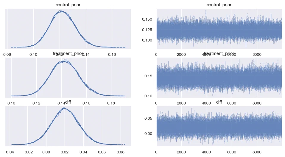

A second plot summarises the posterior functions and difference:

# Plot posterior functions and difference between groups
az.plot_posterior(trace)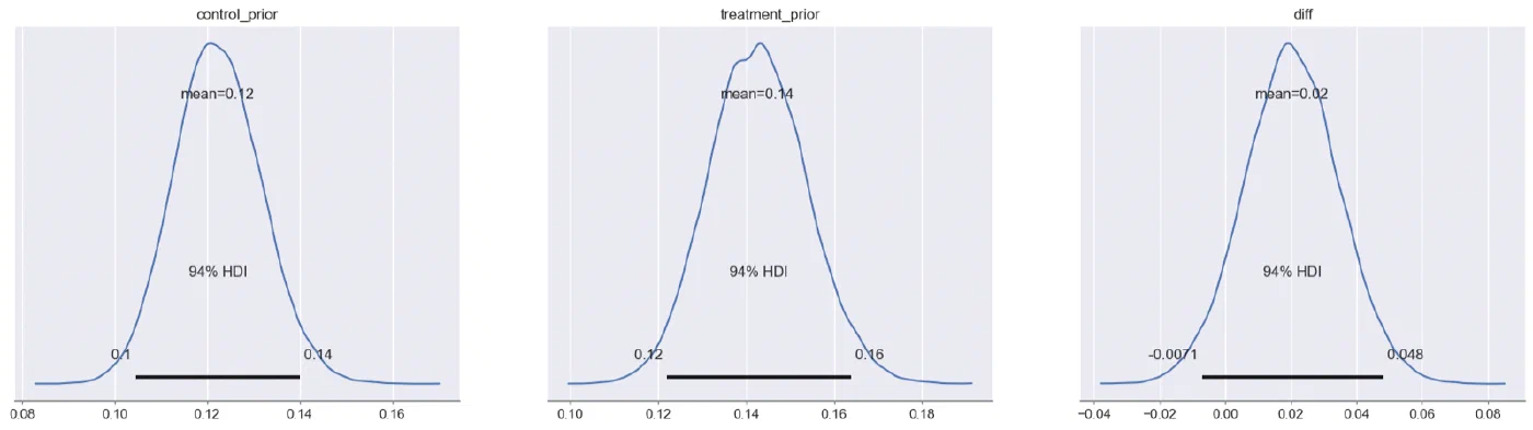

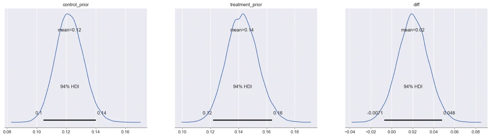
As expected, the 94% Highest Density Interval is close to the 95% Credible Interval that we calculated above.

##Introduction

##Generate sample data

##Frequentist test

##Define prior parameters

##Conjugate distributions

##Assess statistical difference

###Checking fit of posterior functions

###Probability A beats B

###Credible Interval

##Using PyMC