Alpha-spending functions for sequential testing

What is sequential testing?

Standard frequentist tests (like z-tests) assume that data is analyzed all at once, when all data has been collected, a concept referred to as a “fixed horizon”. Peeking, or repeatedly analyzing data during collection, greatly inflates the false positive rate.

To compute intermediary results without this risk, one solution is sequential testing, which allows for data monitoring without inflating Type I error, while detecting early negative impacts on users.

The key principle is to define upper and lower boundaries for the test statistic based on a spending function. Beyond the Bonferroni correction (dividing alpha by the number of planned interim analyses), which is valid but very conservative, several spending functions exist, including Haybittle-Peto (1971, 1976), Pocock (1977), and O’Brien & Fleming (1979). These functions adjust the boundaries depending on the number of interim analyses.

However, they include strict requirements:

The number of scheduled analyses must be determined prior to the onset of the trial.
There must be equal spacing between scheduled analyses with respect to sample size accrual.

Below is a comparison of different methods. The O’Brien & Fleming is much more conservative in earlier steps, while the Pocock function is almost linear.

Source

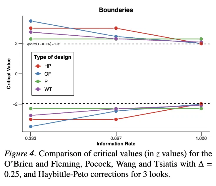
Alpha-spending functions

In 1983, Lan & DeMets developed an approach that removes these constraints, and depends instead on the fraction of information available at each checkpoint. This approach is known as an alpha-spending function.

They approximated the Pocock and O’Brien and Fleming boundaries with this method.

O’Brien and Fleming

Here’s the formula for O’Brien and Fleming approximation for a 1-sided case:

\alpha(t) = 2\left(1 - \Phi\left( \frac{\Phi^{-1}(1 - \frac{\alpha}{2})}{\sqrt{t}} \right)\right)

and for a 2-sided case:

\alpha(t) = 4\left(1 - \Phi\left( \frac{\Phi^{-1}(1 - \frac{\alpha}{4})}{\sqrt{t}} \right)\right)

Pocock

The Lan & DeMets approximation for Pocock boundaries is:

\alpha(t) = \alpha \ln\left(1 + (e - 1) t\right)

where $t$ is the fraction of information available at checkpoint.

Implementation in Python

Let’s implement in Python the Lan & DeMets approximation for O’Brien and Fleming boundaries.

First we import sample data, that gives a daily cumulated number of users and converted users, for Control and Target groups:

# Import libraries
import pandas as pd
import numpy as np
import scipy.stats as st
import statsmodels.stats.proportion as smp
import matplotlib.pyplot as plt
import matplotlib.patches as pltp
import seaborn as sns
sns.set()

# Load sample data
df = pd.read_csv('gst_data.csv')
df.tail(10)

    variant  days  users  converted
44  control    23    985        572
45   target    23   1021        531
46  control    24   1040        604
47   target    24   1067        554
48  control    25   1063        617
49   target    25   1083        561
50  control    26   1092        632
51   target    26   1123        581
52  control    27   1119        647
53   target    27   1159        599

Then we implement the O’Brien and Fleming approximation function, that takes as parameters:

data_fraction: fraction of data at each checkpoint summed over all groups (must be between 0 and 1).
alpha: the $\alpha$ of the desired confidence level
sides: whether it’s a 1- or 2-sided test

The function will return boundaries for both the z-statistic and the alpha level.

# Lan and DeMets approximation for O'Brien and Fleming
def ld_of_bounds(data_fraction, alpha=0.05, sides=2):
    data_fraction = max(0, min(1, data_fraction))
    alpha_bound = sides * 2 * (1 - st.norm.cdf(st.norm.ppf(1 - (alpha / 2) / sides) / np.sqrt(data_fraction)))
    score_bound = st.norm.ppf(1 - alpha_bound / sides)
    return score_bound, alpha_bound

We can also implement the Pocock function, with the same parameters:

# Lan and DeMets approximation for Pocock
def ld_pocock_bounds(data_fraction, alpha=0.05, sides=2):
    alpha_bound = (alpha / sides) * np.log(1+(np.exp(1)-1) * data_fraction)
    score_bound = st.norm.ppf(1 - alpha_bound / sides)
    return score_bound, alpha_bound

Now for each checkpoint - every 2 days in this example - we run a Z-test for proportions, and the boundaries for data fraction at this point, i.e. the cumulated number of users over the pre-defined full sample size:

# Parameters
interim_days = np.arange(1, 28, 2)
full_sample_size = 1100

# Run test at each checkpoint
results_list = []
for i, n in enumerate(interim_days):

    control = df.loc[lambda x: (x['variant'] == 'control') & (x['days'] == n)]
    target = df.loc[lambda x: (x['variant'] == 'target') & (x['days'] == n)]
    count = np.array([target['converted'].sum(), control['converted'].sum()])
    nobs = np.array([target['users'].sum(), control['users'].sum()])
    data_fraction = (target['users'].sum() + control['users'].sum()) / (full_sample_size * 2)
    
    z_stat, p_value = smp.proportions_ztest(count, nobs, alternative='two-sided')
    ## O'Brien & Fleming function
    ld_of = ld_of_bounds(data_fraction)
    ## Pocock function
    ld_pck = ld_pocock_bounds(data_fraction)

    results_list.append({
        'days': n,
        'fraction': data_fraction,
        'z_score': z_stat,
        'p_value': p_value,
        'of_z_bound': round(ld_of[0], 4),
        'of_p_bound': round(ld_of[1], 4),
        'pck_z_bound': round(ld_pck[0], 4),
        'pck_p_bound': round(ld_pck[1], 4),
    })

# Return results
df_bounds = pd.DataFrame(results_list)
print(df_bounds)

days  fraction   z_score   p_value  of_z_bound  of_p_bound  pck_z_bound   pck_p_bound
   1  0.187727 -1.483407  0.137966      5.0422      0.0000       2.6973        0.0070
   3  0.264545 -1.483820  0.137857      4.2036      0.0000       2.5983        0.0094
   5  0.319545 -1.349307  0.177238      3.7965      0.0001       2.5446        0.0109
   7  0.388182 -1.430780  0.152493      3.4130      0.0006       2.4900        0.0128
   9  0.441364 -1.693298  0.090399      3.1781      0.0015       2.4545        0.0141
  11  0.539091 -1.926354  0.054060      2.8383      0.0045       2.4001        0.0164
  13  0.572727 -2.007420  0.044705      2.7414      0.0061       2.3839        0.0171
  15  0.620909 -2.057154  0.039671      2.6160      0.0089       2.3625        0.0182
  17  0.720455 -2.316393  0.020537      2.3966      0.0165       2.3237        0.0201
  19  0.801364 -2.497403  0.012511      2.2481      0.0246       2.2965        0.0216
  21  0.883182 -2.662860  0.007748      2.1182      0.0342       2.2721        0.0231
  23  0.911818 -2.728782  0.006357      2.0768      0.0378       2.2641        0.0236
  25  0.975455 -2.905757  0.003664      1.9910      0.0465       2.2475        0.0246
  27  1.035455 -2.941648  0.003265      1.9600      0.0500       2.2329        0.0256

It looks like the experiment crossed the significance boundaries between days 17 and 19, coincidentally for both Pocock and O’Brien & Fleming functions.

Let’s plot the results, for a clearer view:

# Plot boundaries and results
fig, ax = plt.subplots(1, 2, figsize=(10,4))

## Z-statistics
ax[0].fill_between(df_bounds['days'], -df_bounds['of_z_bound'], df_bounds['of_z_bound'], color='steelblue', alpha=0.2)
ax[0].fill_between(df_bounds['days'], -df_bounds['pck_z_bound'], df_bounds['pck_z_bound'], color='purple', alpha=0.2)
sns.lineplot(data=df_bounds, x='days', y='z_score', marker='.', color='green', ax=ax[0])

## P-values
ax[1].fill_between(df_bounds['days'], -df_bounds['of_p_bound'], df_bounds['of_p_bound'], color='steelblue', alpha=0.2)
ax[1].fill_between(df_bounds['days'], -df_bounds['pck_p_bound'], df_bounds['pck_p_bound'], color='purple', alpha=0.2)
sns.lineplot(data=df_bounds, x='days', y='p_value', marker='.', color='green', ax=ax[1])

## Legend
legend_elements = [
    pltp.Patch(facecolor='steelblue', alpha=0.3, label="O'Brien & Fleming"),
    pltp.Patch(facecolor='purple', alpha=0.3, label='Pocock'),
]
plt.legend(handles=legend_elements, loc='upper right')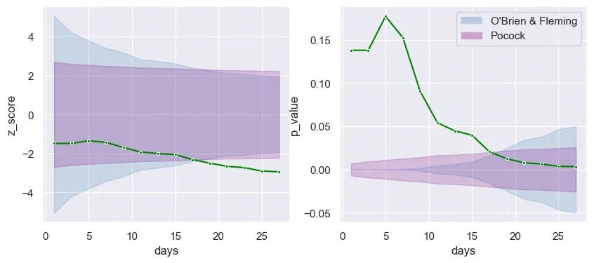

This visually confirms that between day 17 and day 19, the z-score crosses both boundaries, and conversely the p-value enters the boundaries funnel. At this point, we can safely conclude that there is a significant difference between Control and Target groups, and the experiment may be stopped with only 80% of the full sample size.

##What is sequential testing?

##Alpha-spending functions

###O’Brien and Fleming

###Pocock

##Implementation in Python

##Resources

What is sequential testing?

Alpha-spending functions

O’Brien and Fleming

Pocock

Implementation in Python

Resources